Home> Science
Science

By: Claudine Luckett • Science
How To Make Slime Without Glue Or Borax
Introduction Slime has become a popular and fascinating plaything for kids and adults alike. Its stretchy, squishy texture and vibrant colors make it an irresistible sensory experience. While traditional slime recipes call for glue and borax, there are alternative methods to create this gooey delight without these ingredients. Whether you're...
Read More
By: Reena Frisch • Science
The Surprising Truth About Natural Blonde Hair In People Of Color
Introduction Natural blonde hair has long been associated with individuals of European descent, often leading to misconceptions and stereotypes about its rarity in people of color. However, the truth about the presence of blonde hair in diverse ethnicities is a fascinating and often overlooked aspect of human genetics and cultural...
Read More
By: Janine Corcoran • Science
Discover The Surprising Ancestry Connection Revealed By Ancestry DNA Results!
Introduction Embarking on a journey to uncover your ancestral roots is a fascinating endeavor that can unravel a tapestry of connections spanning generations. With the advent of Ancestry DNA testing, individuals are delving into the depths of their genetic makeup to unearth hidden stories and unexpected ties to the past....
Read More
By: Sabra Larosa • Science
The Surprising Truth About Fish And Dehydration – Can They Drown In Water?
Introduction Fish are fascinating creatures that inhabit diverse aquatic environments, captivating the imagination with their vibrant colors and graceful movements. While many people are aware of the importance of water for fish, the concept of fish dehydration might seem perplexing at first glance. In this article, we will delve into...
Read More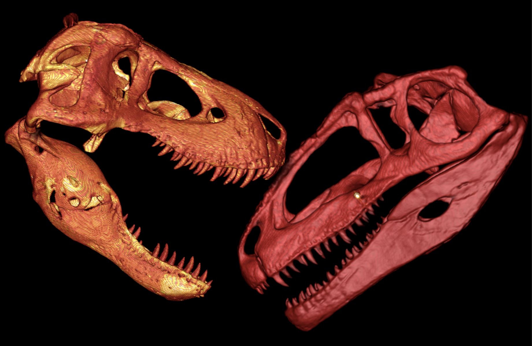
By: Georgie Melson • Science
The Ultimate Battle: T-Rex Vs Giganotosaurus – Who Will Reign Supreme?
Introduction The prehistoric world was once ruled by colossal creatures that roamed the Earth millions of years ago. Among these ancient giants, the Tyrannosaurus rex and the Giganotosaurus stand out as two of the most formidable predators to have ever existed. These apex predators captivate the imagination with their immense...
Read More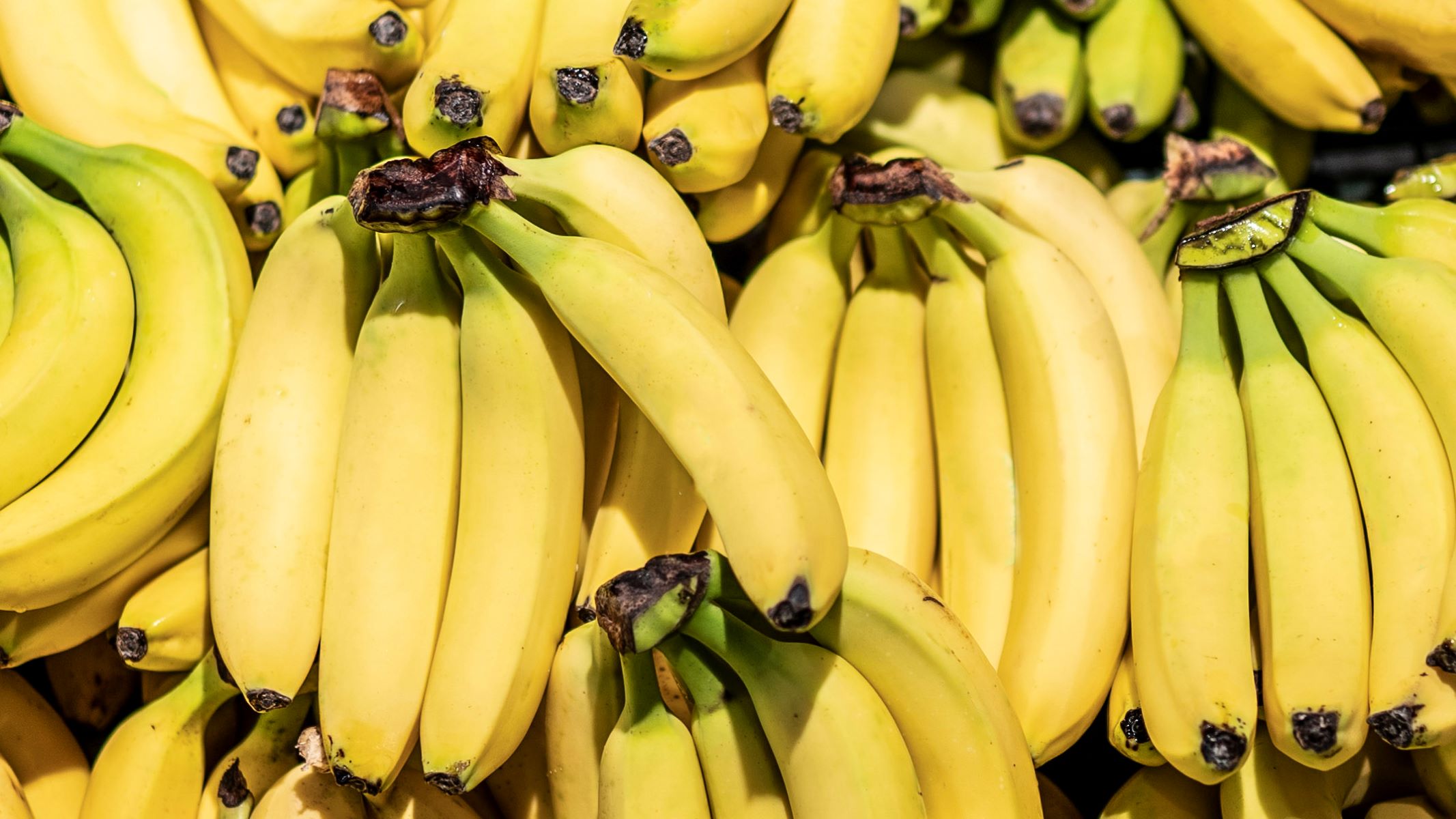
By: Victoria Burt • Science
The Surprising Truth About Bananas – Why They’re Considered Fruits Without Seeds
Introduction Bananas are a beloved fruit enjoyed by people of all ages around the world. Whether sliced over a bowl of cereal, blended into a smoothie, or simply peeled and eaten on the go, bananas have secured their place as a staple in many households. However, have you ever stopped...
Read More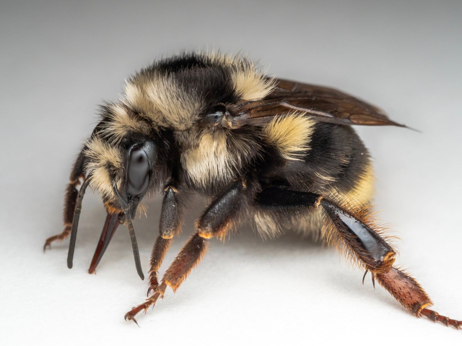
By: Dorette Jurado • Science
Shocking Truth Revealed: The Real Danger Of Black Bumble Bees!
Introduction Bumble bees are often celebrated for their fuzzy appearance and gentle buzzing as they flit from flower to flower, playing a crucial role in pollination. These industrious insects are vital to the health of ecosystems and the success of agricultural crops. However, amidst the vibrant array of bumble bee...
Read More
By: Dynah Cimino • Science
The Surprising Reasons Why 75 Degrees Feels So Different Indoors, Outdoors, And In Water
Introduction Temperature is a fundamental aspect of our daily lives, influencing our comfort, behavior, and overall well-being. Whether we're indoors, outdoors, or submerged in water, the sensation of 75 degrees can vary significantly. This seemingly consistent temperature can evoke distinct perceptions and experiences, prompting us to explore the intriguing science...
Read More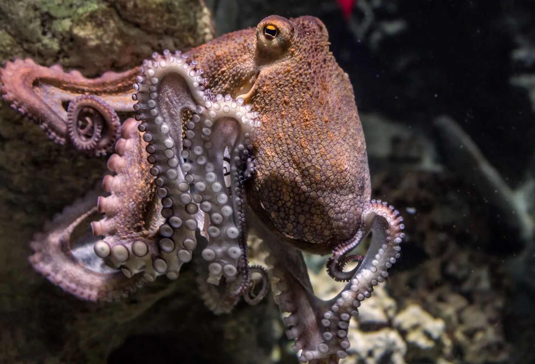
By: Dari Kilburn • Science
The Mind-Blowing Truth: Octopuses Have Multiple Stomachs!
Introduction Octopuses are undoubtedly some of the most fascinating creatures inhabiting our planet. With their remarkable intelligence, shape-shifting abilities, and mesmerizing appearance, these enigmatic creatures have captivated the curiosity of scientists and nature enthusiasts alike. However, one of the most mind-blowing truths about octopuses lies within their digestive system –...
Read More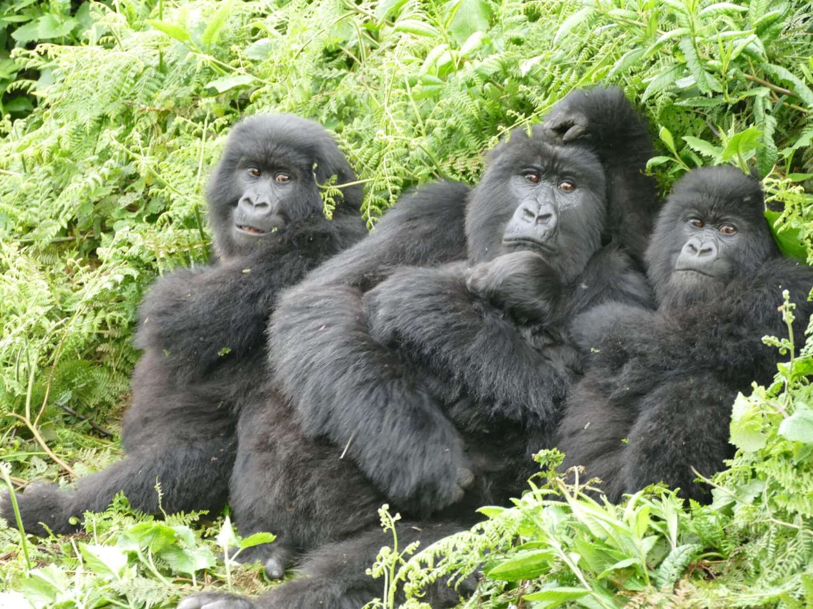
By: Gretchen Roman • Science
The Surprising Source Of Protein For Gorillas Revealed!
Introduction Gorillas, the majestic and powerful primates that roam the dense forests of central Africa, have long captivated the imagination of humans. These gentle giants are known for their impressive strength, imposing presence, and complex social structures. However, one aspect of gorilla life that has puzzled scientists for decades is...
Read More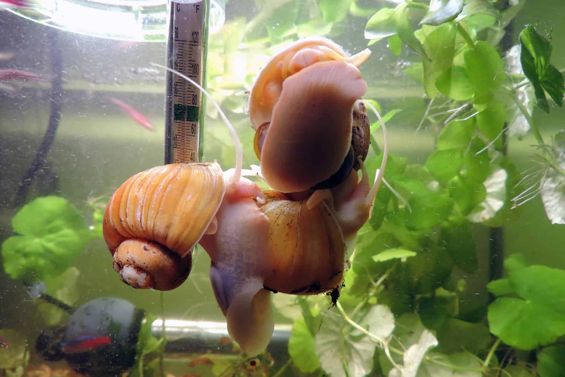
By: Cam Witkowski • Science
Shocking Discovery: The Truth About Your Fish Tank Snail!
Introduction Fish tanks are often a source of tranquility and fascination, providing a glimpse into the mesmerizing underwater world. Among the intriguing inhabitants of these aquatic microcosms are snails. These seemingly innocuous creatures play a crucial role in maintaining the delicate balance of a fish tank ecosystem. However, there are...
Read More
By: Morganne Mcguire • Science
The Surprising Truth About Brown: It’s Actually Dark Green
Introduction Brown is a color often associated with warmth, earthiness, and reliability. It's the color of rich soil, comforting hot cocoa, and the majestic fur of a grizzly bear. But have you ever stopped to ponder the true nature of brown? What if I told you that the color we...
Read More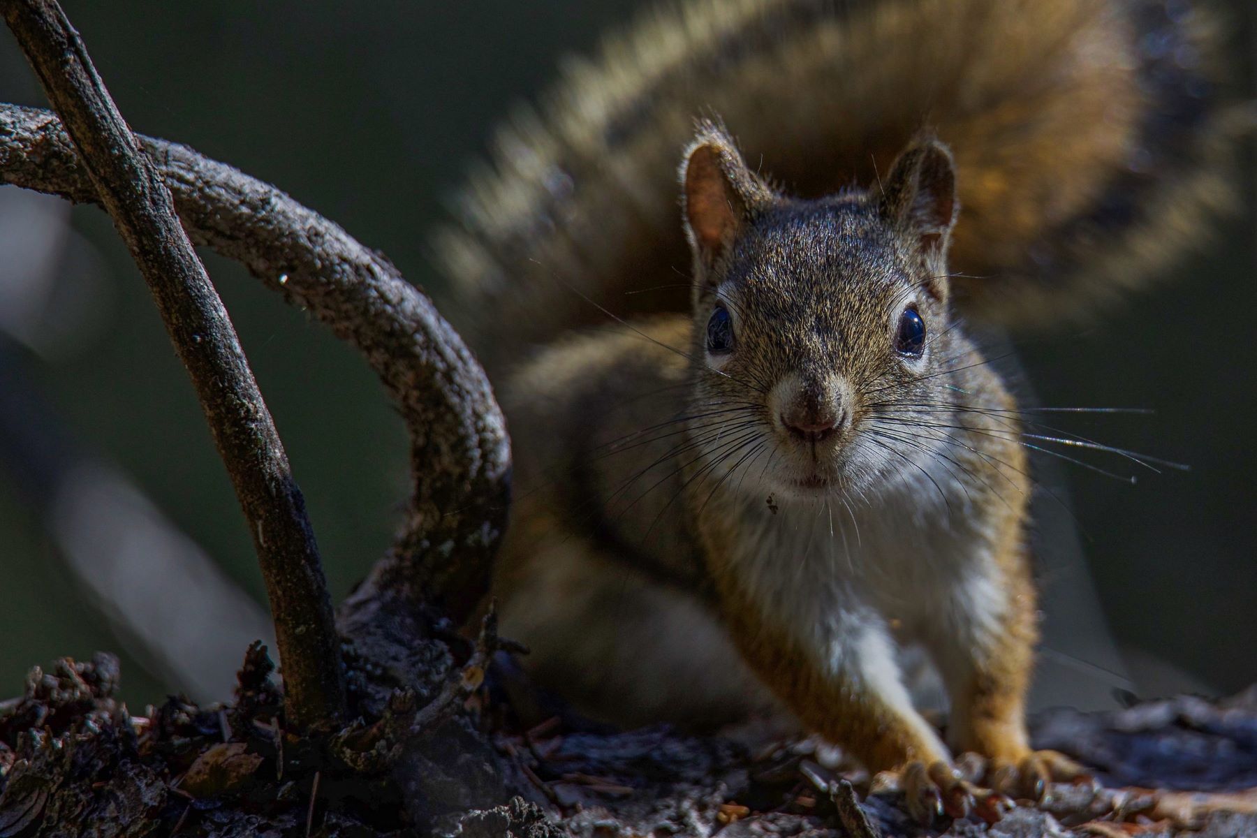
By: Millicent Ezell • Science
The Surprising Reason Why Squirrels Can’t Take Their Eyes Off You
Introduction Squirrels, those ubiquitous and often charming creatures that frolic through parks and scamper up trees, are known for their quick movements and bushy tails. However, have you ever wondered why squirrels seem to have an uncanny ability to fixate their gaze on you, almost as if they are studying...
Read More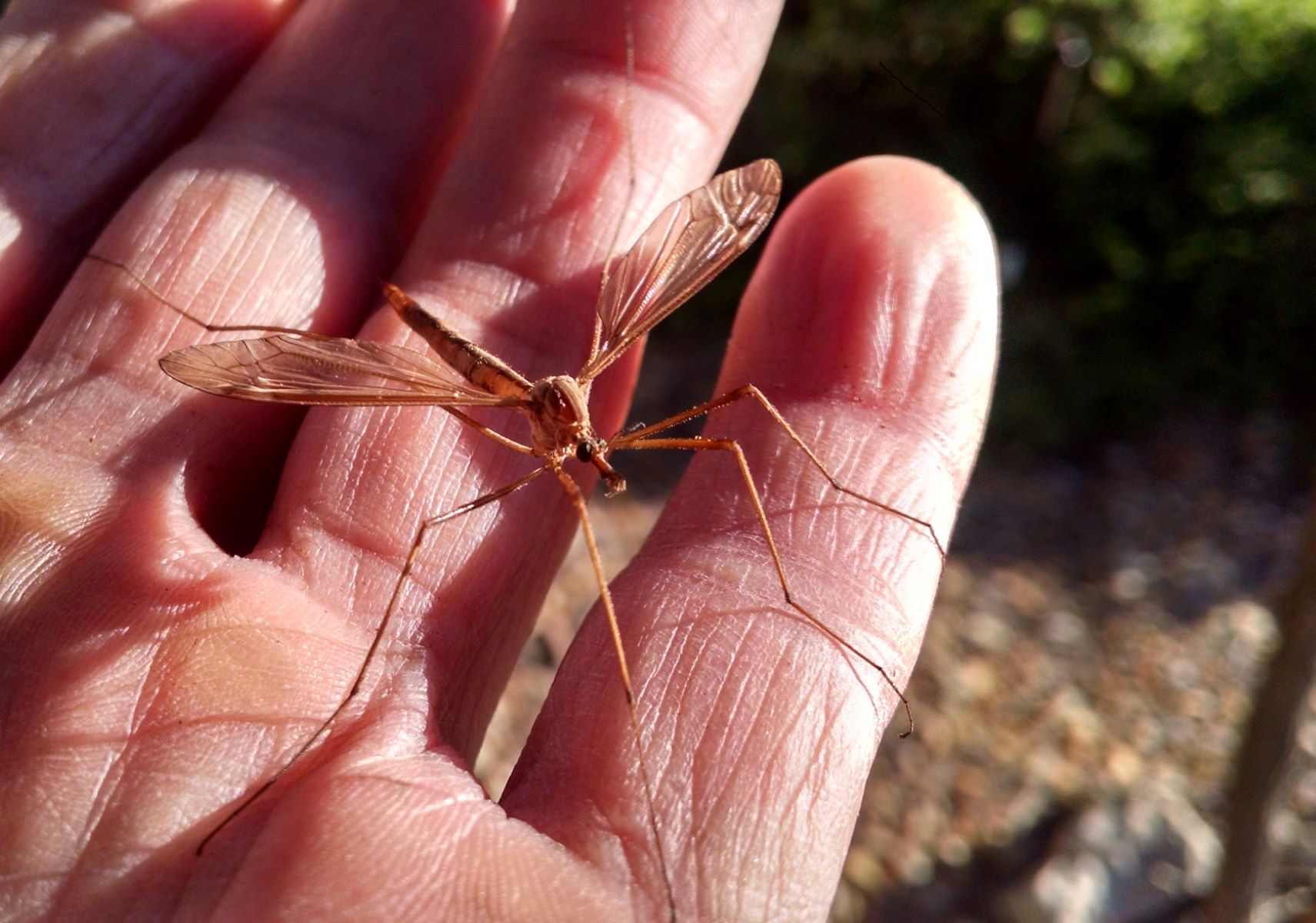
By: Elora Street • Science
Shocking Truth: Mosquito Eaters Vs. Mosquitoes – What You Need To Know!
Introduction Mosquitoes are a familiar nuisance for many, especially during warm summer evenings. Their itchy bites can disrupt outdoor activities and lead to uncomfortable nights. However, there is a common misconception surrounding a group of insects known as "mosquito eaters." These creatures have long been thought to be the natural...
Read More
By: Sheena Coffin • Science
The Surprising Truth: Iron Sharpening Iron In Metallurgy
Introduction The concept of "iron sharpening iron" has long been associated with the process of honing and refining, but its significance extends far beyond the realm of literal metalwork. In metallurgy, the practice of iron sharpening iron involves the use of one iron tool to refine and perfect another, ultimately...
Read More
By: Kevyn Nash • Science
Unbelievable Amp Capacity Of 8-Gauge Copper Wire Revealed!
Introduction Welcome to the world of electrical conductivity and power transmission! In this article, we are about to embark on an enlightening journey into the remarkable realm of 8-gauge copper wire. The astonishing capabilities of this essential component in electrical systems are often overlooked, yet they play a pivotal role...
Read More
By: Lonnie Laws • Science
The Ultimate Ranking: Unveiling The Superior Human Race And The Surprising Decision-Maker!
Introduction In the vast and diverse tapestry of humanity, the concept of superiority has been a subject of fascination and debate for centuries. From the ancient civilizations to the modern era, the quest to understand what defines a superior human has captivated the human mind. This article embarks on a...
Read More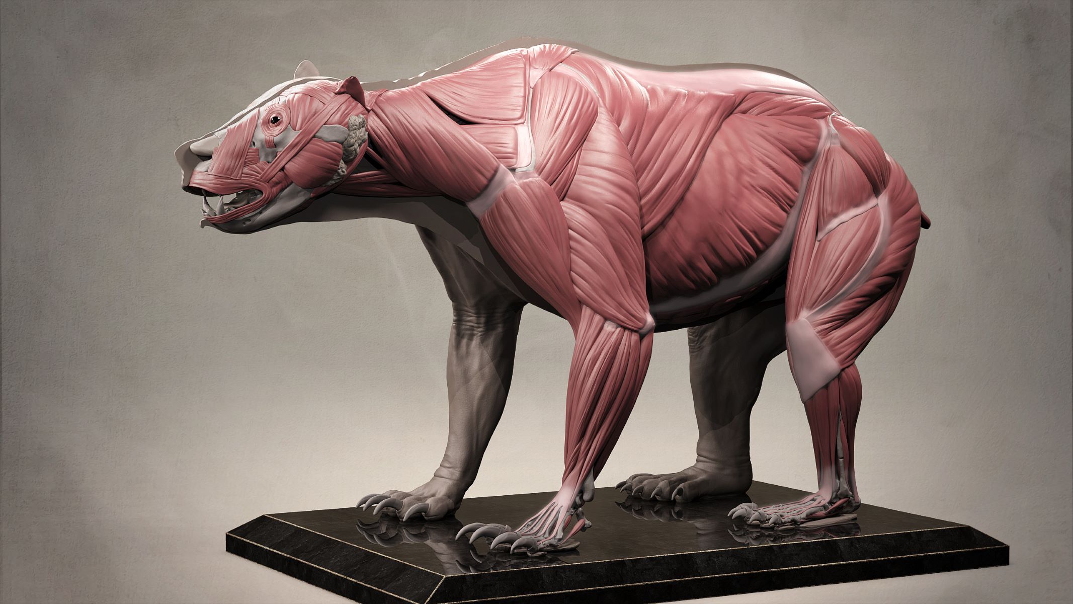
By: Nari Kwon • Science
Unveiling The Astonishing Anatomy Of Bears: Four Legs Or Two Legs And Two Arms?
Introduction Bears have long fascinated and captivated the human imagination with their impressive size, strength, and enigmatic nature. These magnificent creatures are renowned for their remarkable adaptation to various habitats, from the dense forests of North America to the frigid tundra of the Arctic. As we delve into the astonishing...
Read More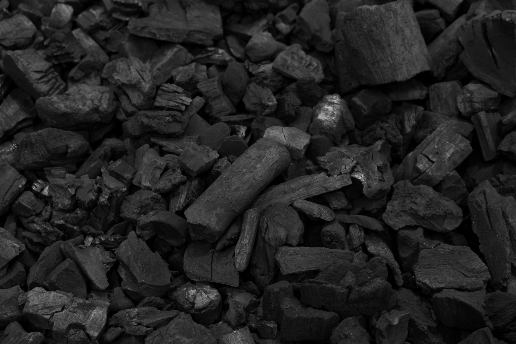
By: Isabelita Fey • Science
The Surprising Truth About Charcoal: Does It Really Last Forever?
Introduction Charcoal is a substance that has been an integral part of human history for millennia. Its uses are diverse, ranging from cooking and heating to industrial applications and art. However, the impact of charcoal production and consumption on the environment has raised concerns in recent years. As we delve...
Read More
By: Giacinta Cheney • Science
Mysterious Invasion: Unveiling The Tiny White Spiders In Your House
Introduction In the quiet corners of many homes, a mysterious invasion often goes unnoticed. Tiny white spiders, barely visible to the naked eye, stealthily navigate their way through the nooks and crannies of our living spaces. These elusive creatures, often overlooked amidst the hustle and bustle of daily life, possess...
Read More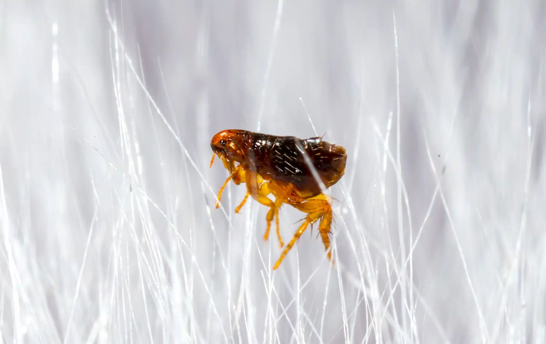
By: Brana Montano • Science
The Surprising Truth About Fleas’ Jumping Abilities
Introduction Fleas are often associated with pesky irritations and relentless itching, but there's more to these tiny creatures than meets the eye. These minuscule insects, known for their incredible jumping abilities, have long piqued the curiosity of scientists and entomologists alike. While their small size may lead one to underestimate...
Read MoreFeatured


By: Doria Ngo • Featured
The Ultimate Guide To Taper Vs. Fade Haircuts: Unveiling The Key Differences
Read More


By: Charlot Alejo • Astrology
The Unconventional Aquarius: Sun, Sagittarius Moon, And Aquarius Rising Revealed!
Read More
PLEATED LAMPSHADE ARE MY NEW FAVORITE THING
SHOULD WE STAY LIGHT OR GO DARK WITH PAINTING OUR TINY MASTER BEDROOM?